The rapid evolution of data analysis and machine learning in modern industries has given rise to advanced methods of interpreting, forecasting, and optimizing processes. Among the various analytical tools available, the Markov model has emerged as a powerful technique for understanding and predicting system behaviours based on probabilistic transitions between states. While initially used in fields such as physics and finance, the Markov model’s utility extends across industries, including procurement, where it is increasingly being adopted to streamline decision-making, improve supply chain management, and reduce risk.
In procurement, understanding supplier behaviour, forecasting demand, managing risks, and optimizing costs are critical. These functions involve analysing vast amounts of data from multiple sources, making it challenging to derive actionable insights using traditional techniques. A Markov model, through its capability to model stochastic processes, provides a robust framework for addressing these challenges.
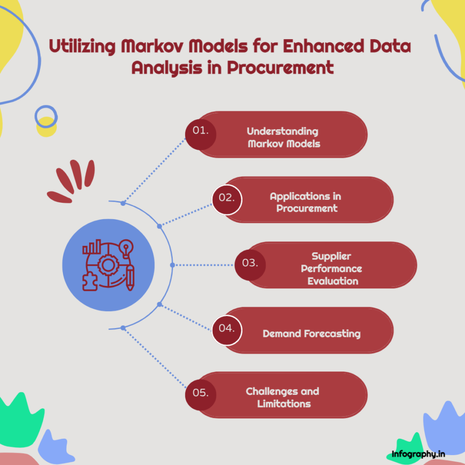
This article aims to explores the Markov model in detail, delving into its mechanics, types, and mathematical foundation. Following that, we will examine its application in procurement, focusing on how it can be used for data analysis in areas such as supplier performance evaluation, risk management, demand forecasting, and cost optimization.
What is a Markov Model?
A Markov model is a mathematical model that represents a system where transitions between states occur based on certain probabilities. The key feature of a Markov model is the Markov property, which states that the future state of the system depends only on the current state, not on the sequence of events that preceded it. This “memoryless” characteristic simplifies the modelling of complex systems, as it reduces the dependencies to just the present state.
In a Markov process, a system moves through a series of states, with each transition determined by a probability. The transitions can be represented as a Markov chain, a sequence of possible events where the probability of each event depends only on the state attained in the previous event.
For a system with a finite number of states, the Markov chain can be described using a transition matrix, which is a square matrix that contains the probabilities of moving from one state to another. The sum of probabilities in each row of the matrix must equal 1, ensuring that the system transitions to one of the possible states at each step.
There are different types of Markov models, including:
- Discrete-time Markov Chains (DTMCs): In a DTMC, the system transitions from one state to another in discrete time steps, with the probabilities of transitions remaining constant over time.
- Continuous-time Markov Chains (CTMCs): In a CTMC, the transitions between states can occur at any point in continuous time, rather than at fixed time steps.
- Hidden Markov Models (HMMs): In an HMM, the states of the system are not directly observable, but they generate observable outputs, allowing for inference about the underlying state based on these outputs.
2. The Mathematical Foundation of Markov Models
The formal structure of a Markov model can be defined as follows:
- Let S={s1,s2,…,sn}S = \{s_1, s_2, …, s_n\} be the set of possible states the system can be in.
- Let PP be the transition matrix, where PijP_{ij} represents the probability of moving from state sis_i to state sjs_j. Thus, PP is an n×nn \times n matrix, and for each row ii, we have:
∑j=1nPij=1\sum_{j=1}^{n} P_{ij} = 1which ensures that the total probability of transitioning to any state from a given state is 1.
- The process starts in an initial state s0s_0, with a given initial probability distribution π0\pi_0, where π0(si)\pi_0(s_i) is the probability that the system starts in state sis_i.
- The state of the system evolves over time steps according to the transition matrix PP. After one step, the probability distribution over the states is π1=π0P\pi_1 = \pi_0 P, and after tt steps, the distribution is πt=π0Pt\pi_t = \pi_0 P^t, where PtP^t is the transition matrix raised to the tt-th power.
Markov models are powerful because they can be used to predict the future state of a system, even with incomplete information, as long as the transition probabilities between states are known or can be estimated.
3. Use Cases of the Markov Model in Data Analysis for Procurement
Procurement is a complex field that involves sourcing goods and services from suppliers, managing supply chains, forecasting demand, and mitigating risks. Decision-makers in procurement rely on data analysis to improve efficiency, reduce costs, and ensure that risks are managed effectively. Here, we will examine several use cases where Markov models can be applied in procurement data analysis.
3.1 Supplier Performance Evaluation
In procurement, managing supplier relationships is crucial to maintaining a reliable supply chain. Supplier performance can vary over time due to changes in production capacity, quality control, or external factors such as economic fluctuations. A Markov model can help track and predict supplier performance by modelling the likelihood of a supplier moving between different performance states, such as “excellent,” “satisfactory,” or “poor.”
By defining these states and estimating the transition probabilities between them, procurement teams can forecast how a supplier’s performance is likely to evolve over time. For example, if a supplier has shown inconsistent quality in recent months, a Markov model might predict the probability that they will continue to underperform or improve their output based on past behavior.
Example:
Consider a supplier that has historically fluctuated between three performance states: high, medium, and low. The transition matrix for this supplier might look like this:
| High | Medium | Low | |
|---|---|---|---|
| High | 0.7 | 0.2 | 0.1 |
| Medium | 0.3 | 0.5 | 0.2 |
| Low | 0.1 | 0.4 | 0.5 |
From this matrix, procurement teams can see that if the supplier is currently in a “High” state, there is a 70% chance they will remain in the high state, a 20% chance they will move to the medium state, and a 10% chance they will drop to the low state. By iterating this process, teams can predict future performance and take proactive measures to mitigate risks, such as identifying alternative suppliers.
3.2 Risk Management in Supply Chain
One of the key challenges in procurement is managing supply chain risks. External factors, such as geopolitical tensions, natural disasters, or financial instability, can disrupt supply chains, leading to delays or shortages. A Markov model can be used to assess the probability of different risk events occurring and their potential impact on the procurement process.
By modelling various risk states (e.g., “normal operation,” “minor disruption,” “major disruption”) and estimating the likelihood of transitions between these states, procurement teams can develop contingency plans and mitigate risks more effectively.
For example, a Markov model could be used to estimate the probability of a major supplier experiencing a disruption in production due to geopolitical events. Based on historical data, procurement managers could estimate how likely it is that the supplier will remain in a stable state versus entering a disruption phase. This allows for more informed decision-making, such as pre-emptively sourcing alternative suppliers or increasing inventory in anticipation of potential disruptions.
3.3 Demand Forecasting
In procurement, accurately forecasting demand is essential for managing inventory levels and ensuring that supply meets demand without overstocking. Demand often fluctuates due to seasonal trends, market conditions, or changes in consumer preferences. A Markov model can be employed to forecast demand by modelling the transitions between different demand states over time.
For example, a retail company might classify demand into three states: low, medium, and high. The company can then estimate the probabilities of moving between these states based on historical sales data. By doing so, the company can predict future demand patterns and adjust procurement strategies accordingly, such as ordering more stock when the likelihood of moving to a “high demand” state increases.
Example:
Let’s assume a product has the following demand transition probabilities:
| Low | Medium | High | |
|---|---|---|---|
| Low | 0.6 | 0.3 | 0.1 |
| Medium | 0.2 | 0.6 | 0.2 |
| High | 0.1 | 0.4 | 0.5 |
If demand is currently low, there is a 60% chance it will remain low, a 30% chance it will rise to medium, and a 10% chance it will increase to high. By using this model, the procurement team can prepare for possible demand fluctuations, ensuring optimal inventory levels and avoiding both stockouts and excess stock.
3.4 Cost Optimisation
Procurement often involves negotiating prices with suppliers, managing budgets, and optimizing costs. Markov models can be used to analyse price trends and forecast future pricing scenarios. By modelling price states (e.g., “low,” “medium,” and “high”) and the transition probabilities between these states, procurement teams can anticipate future price movements and make strategic purchasing decisions.
For instance, if historical data shows that the price of a key raw material tends to fluctuate between different states, a Markov model can be used to predict the probability that the price will rise or fall in the near future. This information can guide procurement teams in deciding whether to lock in prices through long-term contracts or wait for prices to decrease.
4. Implementing a Markov Model in Procurement Data Analysis
Implementing a Markov model in procurement data analysis requires several key steps:
Define the States: The first step is to define the states that represent different conditions of the system you are modelling. For example, in supplier performance evaluation, the states might be “high performance,” “medium performance,” and “low performance.”
Estimate Transition Probabilities: Once the states are defined, the next step is to estimate the probabilities of transitioning between states. This can be done using historical data or expert judgment. For example, if a supplier has moved from “high” to “medium” performance in 20% of the observed periods, the transition probability from “high” to “medium” would be 0.2.
Build the Transition Matrix: With the transition probabilities estimated, you can construct the transition matrix, which describes how the system moves from one state to another.
Predict Future States: After building the transition matrix, you can use it to predict future states. This can be done by multiplying the initial probability distribution by the transition matrix, iterating over multiple time steps to forecast the
future state of the system. For example, if you are evaluating supplier performance, you can estimate the likelihood of a supplier improving, maintaining, or declining in performance over a given period. By iterating the transition matrix over time, you can forecast several future periods and adjust your procurement strategy accordingly.
Validate the Model: Once predictions are made, it’s crucial to validate the model using real-world data. If the model’s predictions align closely with actual outcomes, you can be confident in its accuracy. If not, you may need to adjust the states or transition probabilities based on additional data or insights.
Incorporate External Factors: While the Markov model is powerful for representing stochastic processes, it may be limited if there are significant external factors that influence state transitions. For instance, economic conditions, political changes, or sudden shifts in demand can all impact procurement outcomes. Integrating external data into the model can improve its predictive capabilities and make it more robust.
5. Real-World Example: Using Markov Models in Supplier Performance Analysis
To illustrate how Markov models can be used in procurement, let’s explore a real-world scenario where a procurement department monitors supplier performance using a Markov model.
Scenario: A large retail company sources products from multiple suppliers. Each supplier is evaluated on three key performance metrics: quality of goods, on-time delivery, and price consistency. The suppliers are categorized into three performance states: “excellent,” “average,” and “poor.” Over time, the company collects performance data and builds a Markov model to predict how supplier performance may change.
State Definition:
- State 1: Excellent performance (high quality, on-time delivery, stable pricing)
- State 2: Average performance (acceptable quality, occasional delays, price fluctuations)
- State 3: Poor performance (low quality, frequent delays, volatile pricing)
Building the Transition Matrix: Based on historical performance data, the procurement team estimates the following transition probabilities between the states:
Excellent (S1) Average (S2) Poor (S3) S1 0.8 0.15 0.05 S2 0.3 0.5 0.2 S3 0.1 0.4 0.5 In this matrix, each row sums to 1, representing the total probability of transitioning from one state to any other state, including remaining in the same state.
Analysing the Transition Matrix:
- If a supplier is currently in the “Excellent” state (S1), there is an 80% chance they will stay in the excellent state, a 15% chance they will degrade to “Average,” and a 5% chance they will drop to “Poor.”
- If a supplier is in the “Poor” state (S3), they have a 50% chance of remaining poor, a 40% chance of improving to “Average,” and a 10% chance of jumping to “Excellent.”
Prediction Over Time: The procurement team can now predict supplier performance over several time periods. If the initial probability distribution is that 70% of suppliers are in the “Excellent” state, 20% in “Average,” and 10% in “Poor,” they can forecast the distribution of suppliers’ future performance after, say, three time periods.
By multiplying the initial probability distribution by the transition matrix raised to the third power, the procurement team could predict the expected distribution of suppliers in each state after three periods.
Decision-Making and Strategy: Based on these forecasts, the procurement team can make strategic decisions. If a large portion of suppliers is expected to drop from “Excellent” to “Average,” the team might decide to proactively seek new suppliers or renegotiate contracts. Conversely, if most suppliers are expected to remain in the “Excellent” state, the team can focus on strengthening relationships with these suppliers, ensuring long-term partnerships.
6. Hidden Markov Models (HMM) for Procurement Applications
While traditional Markov models are effective for modelling visible transitions between states, there are cases in procurement where the state of the system is not directly observable. For example, the financial health of a supplier or the likelihood of supply chain disruption may not be immediately apparent from observable data. In such cases, Hidden Markov Models (HMMs) can be useful.
In an HMM, the system passes through a series of hidden states, but each hidden state produces observable outputs. By analysing these outputs, it is possible to infer the underlying hidden states and make predictions about future behaviour.
Application Example: Supplier Financial Health Monitoring
Consider a scenario where a company wants to monitor the financial health of its suppliers but only has access to indirect data such as delivery performance, order fulfilment times, and pricing trends. While this data doesn’t directly reveal the financial health of the supplier, it can serve as an observable output of an HMM.
Hidden States: These might represent the financial condition of the supplier:
- State 1: Strong financial health
- State 2: Moderate financial health
- State 3: Poor financial health
Observations: The procurement team collects observable data, such as:
- Delivery delays
- Price fluctuations
- Customer complaints
Building the HMM: By analysing the observable outputs, the procurement team can estimate the probabilities that a supplier is in one of the hidden states. For example, a supplier with increasing delivery delays and price instability may have a high probability of being in the “poor financial health” state.
Risk Management: Once the HMM is built, the procurement team can use it to predict the likelihood of suppliers moving between different financial states. This allows for early intervention and risk mitigation. For example, if a key supplier is likely to enter a state of poor financial health, the procurement team can proactively source alternative suppliers to avoid supply chain disruptions.
7. Limitations of Markov Models in Procurement
While Markov models offer valuable insights for procurement analysis, there are certain limitations to consider:
Markov Property Assumption: Markov models assume that the future state depends only on the current state, not on the sequence of events that preceded it. In reality, procurement processes can be influenced by long-term trends and historical factors, making the Markov property an imperfect assumption.
Data Availability: Accurate estimation of transition probabilities requires large amounts of historical data. If sufficient data is not available, the reliability of the model’s predictions may be compromised.
Complexity of Procurement Systems: Procurement is influenced by numerous internal and external factors, such as market dynamics, geopolitical risks, and regulatory changes. While Markov models can capture some of these complexities, they may oversimplify others.
External Influences: Markov models do not always account for external shocks, such as sudden economic downturns, that can significantly affect supplier performance and demand patterns. Hybrid models that combine Markov processes with other forecasting methods may be needed to handle such events.
Here are some useful sources for understanding Markov models and their application, especially within procurement and related fields:
Fundamentals of Markov Analysis: Theory & Industry Use-cases
This source discusses the core principles of Markov models, including how they can be used across various industries like human resources, engineering, and procurement. The article provides insights into how Markov models are applied to predict system transitions and how this method simplifies prediction by relying on current state data.
URL: www.markovml.comMarkov Models Related to Inventory Systems, Control Charts, and Forecasting Methods
This source explores the application of Markov models in supply chain management, particularly in inventory control and queuing systems. It provides practical examples of Markov models in procurement-related tasks like managing inventory levels and minimizing costs.
URL: www.intechopen.comProcurement Analytics: Data-Driven Decision-Making in Procurement and Supply Management
This textbook highlights how advanced analytics, including Markov models, are used in procurement to generate economic value by reducing costs and managing risks. It discusses the intersection of data science and procurement, including topics such as spend management, supplier management, and risk management.
URL: SpringerLinkMarkov Analysis: Insights, Applications, and Real-World Examples
This article provides an overview of how Markov models are applied across various industries, including their role in procurement for risk management and resource allocation. It discusses challenges, emerging trends, and practical tips for implementing Markov models in dynamic environments.
URL: SuperMoneyProcurement Analytics: The Ultimate Guide in 2024
This guide explains how procurement analytics, including techniques like Markov modelling, helps organizations manage supply chains, reduce costs, and mitigate risks. It also touches on how Markov models contribute to supplier performance monitoring and demand forecasting in procurement.
URL: Sievo
Power BI doesn’t have a built-in Markov model function. Here’s a high-level approach to implementing a Markov model based on sales data, including Sales Value, Product Code, Date of Purchase, and Quantity Purchased:
1. Step 1: Organize Data into States
In a Markov model, you need to define the “states” of your system. For a sales dataset, the states could represent sales value categories (e.g., low, medium, high), product categories, or buying frequency patterns.
- For example, you can define states based on sales value ranges like:
- Low Sales: Sales Value between $0 and $100
- Medium Sales: Sales Value between $101 and $500
- High Sales: Sales Value above $500
You will then need to categorize the sales values into these states. You can create a calculated column for this in DAX, such as:
SalesState =
SWITCH(
TRUE(),
Sales[SalesValue] < 100, "Low",
Sales[SalesValue] <= 500, "Medium",
"High"
)
2. Step 2: Create Transition Matrix
In a Markov model, you calculate the probabilities of transitioning from one state to another. In Power BI, you would need to track the purchases over time and count the transitions between states (e.g., from “Low” sales in one period to “Medium” sales in the next).
First, create a calculated column to rank the purchase orders by Date of Purchase for each Product Code:
OrderRank =
RANKX(
FILTER(Sales, Sales[ProductCode] = EARLIER(Sales[ProductCode])),
Sales[DateOfPurchase],,
ASC
)
Next, create a calculated column to capture the state of the previous purchase:
PreviousSalesState =
CALCULATE(
MAX(Sales[SalesState]),
FILTER(Sales,
Sales[ProductCode] = EARLIER(Sales[ProductCode]) &&
Sales[OrderRank] = EARLIER(Sales[OrderRank]) - 1
)
)
This column captures the sales state of the previous purchase for each product.
3. Step 3: Calculate Transition Probabilities
You will now count how many times each transition occurs and then calculate the transition probabilities. For example, count how many times a “Low” state transitions to a “Medium” state.
Create a measure to count transitions between states:
TransitionCount =
CALCULATE(
COUNTROWS(Sales),
Sales[SalesState] = "Medium" && Sales[PreviousSalesState] = "Low"
)
You can create similar measures for other transitions (e.g., from “Medium” to “High”).
Next, calculate the transition probabilities by dividing the number of transitions from one state to another by the total transitions out of the initial state:
TransitionProbability =
DIVIDE(
[TransitionCount],
CALCULATE(COUNTROWS(Sales), Sales[PreviousSalesState] = "Low")
)
4. Step 4: Predict Future States
Using the transition probabilities, you can predict the future state by multiplying the current state’s distribution by the transition matrix. This is more complex to implement directly in DAX, but you can calculate an approximation by applying the transition probabilities to the current state distribution.
While Power BI doesn’t natively support complex algorithms like Markov models, DAX can be used to build a simplified version by defining states, calculating transitions, and estimating probabilities. This approach, although manual, allows you to model customer purchase behaviour and predict future states based on historical data. For more complex Markov chain implementations, you might consider integrating Power BI with Python or R scripts, which are better suited for matrix calculations and stochastic processes.
The Markov model is a powerful tool for data analysis in procurement, offering a way to model and predict the behaviour of systems that evolve over time in uncertain environments. By applying Markov models to supplier performance evaluation, risk management, demand forecasting, and cost optimization, procurement teams can make more informed decisions and develop more robust strategies.
However, the effectiveness of Markov models in procurement depends on the availability of reliable data and the appropriate definition of states and transitions. In some cases, integrating external factors or employing more complex models such as Hidden Markov Models (HMMs) may be necessary to capture the full complexity of procurement processes.
As data analysis continues to evolve, the use of Markov models in procurement is likely to grow, providing new opportunities for organizations to optimize their supply chains, manage risks, and reduce costs. By understanding the strengths and limitations of Markov models, procurement professionals can harness their potential to drive better outcomes in an increasingly complex and dynamic business environment.